Duplicate records appear inside workbooks through manual data entry, overlapping software imports, and combined departmental exports. When identical rows linger inside inventory sheets, payroll summaries, or customer contact books, report summaries calculate inaccurate figures, VLOOKUP functions pull wrong targets, and accounting balances fall out of alignment. Cleaning spreadsheets correctly requires understanding when to highlight values for human review, when to filter rows non-destructively, and when to execute permanent row deletions.
Quick Action Summary
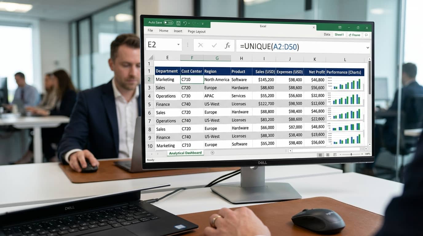
To delete identical rows immediately, select your dataset and press Alt + A + M on your keyboard. Select your target columns and click OK. To preserve your original records without risk of data loss, extract clean unique rows into adjacent columns using the formula =UNIQUE(A2:D500).
Exact Matches vs Primary Key Duplicates
Before executing any cleanup operation, you must examine how your data defines an invalid duplicate. Duplicate records fall into two distinct structural categories within business spreadsheets:
- Full-Row Matches: Every single cell in row 12 matches row 45 from column A through column Z. These instances almost always represent accidental double entry, faulty copy paste actions, or repetitive database extracts. Removing them preserves overall integrity.
- Partial Key Matches: Two rows share an identical Customer ID, Email Address, or Serial Code, yet differ in order timestamp, shipping status, or transaction total. Purging one of these rows based solely on the identifier column erases legitimate financial transactions or historical customer notes.
Prior to deleting rows permanently, create a safety copy of your active worksheet. Right-click the worksheet tab at the bottom of Excel, choose Move or Copy, check the box labeled Create a copy, and click OK. Having an unaltered baseline prevents disastrous data loss if you inadvertently remove valid customer transactions.
When managing client databases or operational lists where immediate deletion could risk destroying context, visual inspection provides safety. Conditional formatting highlights matching cells so your team can verify entries before taking destructive actions.
- Select the column containing the primary values you want to inspect (for example, column B containing email addresses).
- Navigate to the Home tab on the Excel ribbon.
- Click on Conditional Formatting inside the Styles section.
- Hover over Highlight Cells Rules and choose Duplicate Values from the submenu.
- In the prompt that appears, confirm that the first dropdown box displays Duplicate.
- Choose your preferred formatting appearance from the right-hand dropdown, such as Light Red Fill with Dark Red Text or a custom soft yellow highlight.
- Click OK to apply the rule across your range.
Once the formatting rule illuminates matching records, sort your sheet by color to group duplicate values together. Click any cell within your data range, open the Data tab, click Sort, pick your key column, change the Sort On parameter to Cell Color, and choose your highlight shade. This surfaces all matching values directly at the top of your sheet for rapid side-by-side comparison.
Workbook Speed Advisory: Conditional formatting evaluates continuously inside Excel memory. When applied across tables containing more than 20,000 rows, sheet scrolling becomes sluggish and formula calculations slow down. Clear highlighting rules via Home > Conditional Formatting > Clear Rules once visual inspection finishes.
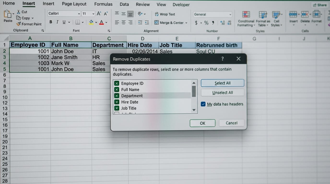
Once you have audited your records and want to purge redundant rows permanently, the native Excel deduplication tool is the fastest method available. It scans your chosen range and deletes subsequent copies of each identified record while keeping the earliest occurrence intact.
- Click any single cell inside your data grid. Excel automatically detects adjacent populated rows and columns.
- Navigate to the Data tab on the ribbon and locate the Data Tools section.
- Click the Remove Duplicates button, or press keyboard shortcut Alt + A + M.
- Confirm that the checkbox labeled My data has headers accurately reflects whether your top row holds column titles. Leaving this unchecked will accidentally include your header text in the deduplication scan.
- Determine which columns establish a match. If you click Select All, Excel only deletes rows where every single cell across every column matches another row. If you check only Email, Excel keeps the first instance of each email address and deletes every following row with that email, regardless of differences in phone numbers or dates.
- Click OK. An alert box appears displaying the exact count of duplicate rows eliminated and the count of unique rows retained.
Be aware that Excel retains the top-most record and deletes everything below it. If your dataset contains chronological updates where the latest row sits at the bottom, sort your data by date descending before initiating this tool to ensure you retain the newest record rather than the oldest entry.
Users working in current spreadsheet editions such as Excel 365, Excel 2021, and Excel for the Web can use dynamic array formulas. Unlike destructive buttons that modify source grids permanently, formula isolation outputs clean tables into empty cells while keeping source rows unchanged.
The base syntax for isolating unique records follows this structure:
=UNIQUE(array, [by_col], [exactly_once])
Here is how each parameter functions:
array: The range of rows and columns containing your data (for example, A2:D500).[by_col]: Optional. Enter FALSE to compare row by row (standard vertical behavior), or TRUE to compare column by column. Default is vertical comparison.[exactly_once]: Optional. Enter FALSE to return all distinct values (the common deduplication goal). Enter TRUE if you want to isolate only records that appeared once, fully excluding any item that had a repeat.
To create a presentation-ready summary report that filters out empty rows and sorts results alphabetically, nest the function inside SORT and FILTER:
=SORT(UNIQUE(FILTER(A2:D500, A2:A500<>"")))
Whenever team members add new rows to your raw input range, this formula automatically recalculates and adds new unique entries into your output table. If you see a #SPILL! error, clear any existing text, formulas, or formatting from the cells directly below and to the right of your formula cell to allow the dynamic array room to expand.
Automated Cleansing with Power Query
If you clean regular monthly transaction exports from enterprise software systems, repeating manual menu clicks wastes valuable operational hours. Power Query provides an automated data pipeline that saves cleanup steps and reruns them whenever source files refresh.
- Highlight your source data and click Data > From Sheet (or From Table/Range).
- If your data is not yet formatted as an official table, Excel prompts you to create one. Click OK. The Power Query Editor window launches.
- To eliminate full-row identical records, click the small table icon in the upper-left corner of the data preview grid and select Remove Duplicates. This writes the function
Table.Distinct(#"Changed Type") into your query steps.
- To eliminate duplicates based on a single identifier column such as Account Number, select that column header, right-click, and select Remove Duplicates. Power Query will evaluate records strictly against that specific field.
- Click the Close & Load button on the Home ribbon of the Power Query Editor. Excel streams the cleaned dataset into a brand new worksheet tab.
Next week, when you drop updated sales rows into the original table, simply navigate to the output sheet, right-click any cell, and hit Refresh. Power Query automatically applies your deduplication logic in seconds without requiring formula adjustments or manual dialog configurations.
Flagging Duplicates with the COUNTIF Formula
When you need to keep your dataset intact but need to categorize each record as either an original entry or a duplicate occurrence, an expanding COUNTIF helper column provides full visibility.
Insert a new column next to your data called Duplicate Status. In cell E2, type this expanding range formula and drag it down:
=IF(COUNTIF($A$2:A2, A2)>1, "Duplicate", "Original")
Notice the critical placement of dollar signs in the formula syntax. The absolute reference $A$2 locks the top starting boundary, while the relative reference A2 expands as the formula fills downward.
- The first time a value appears in row 2, the formula counts exactly 1 occurrence within
$A$2:A2 and returns Original.
- When that same value reappears in row 84, the formula counts 2 occurrences within
$A$2:A84 and returns Duplicate.
- If it reappears in row 120, the count reaches 3, continuing to return Duplicate.
You can now apply standard AutoFilters (Ctrl + Shift + L), filter your helper column to display only "Duplicate", and review or delete those specific rows safely.
Batch Deduplication Using VBA Macros
For system administrators and analysts who process hundreds of repetitive CSV files daily, Visual Basic for Applications (VBA) executes deduplication instantly without manual interaction. Press Alt + F11 to open the VBA Editor, insert a new standard module, and paste this production script:
Sub BatchRemoveDuplicates()
    Dim targetSheet As Worksheet
    Dim lastRowNumber As Long
    Dim lastColNumber As Long
    Dim sourceDataRange As Range

    ' Optimize execution speed by suppressing screen flicker
    Application.ScreenUpdating = False
    Application.Calculation = xlCalculationManual

    Set targetSheet = ActiveSheet
    lastRowNumber = targetSheet.Cells(targetSheet.Rows.Count, "A").End(xlUp).Row
    lastColNumber = targetSheet.Cells(1, targetSheet.Columns.Count).End(xlToLeft).Column

    If lastRowNumber > 1 Then
        Set sourceDataRange = targetSheet.Range(targetSheet.Cells(1, 1), targetSheet.Cells(lastRowNumber, lastColNumber))

        ' Purge duplicates based on Column 1 (Primary Key)
        sourceDataRange.RemoveDuplicates Columns:=Array(1), Header:=xlYes

        Dim remainingRows As Long
        remainingRows = targetSheet.Cells(targetSheet.Rows.Count, "A").End(xlUp).Row

        MsgBox "Data cleanup finished. Active table now contains " & remainingRows & " total rows.", vbInformation, "Clean Finished"
    Else
        MsgBox "No data records detected for deduplication.", vbExclamation, "Empty Dataset"
    End If

    ' Restore default Excel application states
    Application.Calculation = xlCalculationAutomatic
    Application.ScreenUpdating = True
End Sub
This script turns off display refreshes and calculation engines during execution, allowing it to process sheets with over 100,000 rows in just a few seconds without crashing Excel.
Method Comparison: Speed vs Data Safety
Selecting the best deduplication method depends on whether you need a quick manual cleanup, non-destructive formula extraction, or an automated pipeline for massive workbooks:
| Cleanup Method |
Execution Speed |
Destructive to Data? |
Dynamic / Auto-Updating |
Best Operational Scenario |
| Native Remove Duplicates Tool |
Instant |
Yes (Deletes rows) |
Static (Manual run) |
One-off contact lists, standalone exports |
| Dynamic UNIQUE Formula |
Real-Time |
No (Preserves raw data) |
Automatic on recalculation |
Reporting dashboards, dependent summaries |
| Conditional Formatting |
Fast |
No (Highlights only) |
Automatic display rule |
Visual auditing before taking destructive steps |
| Power Query ETL Pipeline |
Moderate |
No (Clean output table) |
Refreshable on click |
Recurring monthly accounting and ERP files |
| VBA Macro Routine |
Fast on 100k+ rows |
Customizable |
Triggered via button |
High-volume enterprise workbook automation |
Troubleshooting Whitespace, Case Sensitivity, and Number Formats
When Excel reports that no duplicates were found, yet your eyes see identical words right next to each other, hidden character discrepancies are preventing clean matches. Here are three proven troubleshooting fixes:
1. Stripping Invisible Trailing Spaces and Non-Breaking Characters
Web scrapers, online forms, and database extracts routinely append trailing spaces or non-breaking web spaces (ASCII code 160). To Excel, the text "Server01" and the text "Server01 " represent two completely different strings. Standard TRIM functions only strip regular ASCII 32 spaces, leaving non-breaking spaces intact. Use this formula in a helper column to scrub entries thoroughly:
=TRIM(CLEAN(SUBSTITUTE(A2, CHAR(160), " ")))
2. Fixing Number Stored as Text Mismatches
If one software system exports invoice numbers as pure numbers (e.g., 90412) and another exports them as text strings (e.g., '90412), Excel will never match them as duplicates. Standardize your columns by selecting the text column, opening the Data tab, clicking Text to Columns, and immediately clicking Finish without altering default delimiters. Excel immediately converts text numbers into true numeric values.
3. Enforcing Case-Sensitive Deduplication
Because Excel built-in deduplication is strictly case-insensitive, values like "NYC" and "nyc" are treated as identical duplicates. If your system requires preserving case sensitivity (such as case-sensitive API tokens, security hashes, or product SKU codes), use an exact comparison formula:
=IF(SUMPRODUCT(--EXACT($A$2:A2, A2))>1, "Duplicate", "Unique")
The EXACT function checks character case strictly, while the double unary operator (--) converts TRUE and FALSE evaluations into 1 and 0 for accurate mathematical counting.
4. The First-Occurrence Deletion Trap (Keeping the Latest Record)
Excel built-in deduplication always preserves the first physical row and deletes every duplicate row below it. If your workbook is logged chronologically with timestamps, running Remove Duplicates deletes your most recent customer update or newest inventory count, leaving outdated records behind.
To ensure Excel keeps the newest entry, sort your dataset by date or order ID in Descending Order (Newest to Oldest) before pressing Alt + A + M. This positions your freshest data at the top, guaranteeing that Excel preserves the correct record while purging historical duplicates.
Once your dataset is scrubbed of redundant records, maintaining data integrity requires preventing future typographical errors at the entry point. A proven best practice is standardizing user input with an Excel drop-down list, which restricts input cells to approved items. For executive dashboards and status summaries derived from cleaned unique rows, you can also format your records clearly by learning how to add bullet points in Excel for organized single-cell notes.